Neural Radiance Fields and Volume Rendering

This post aims to explain how neural radiance fields (NeRFs) work. The original NeRF paper was released in 2020 by researchers at UC Berkeley, Google Research, and UC San Diego. Since then, there has been a lot of follow up work improving on and involving NeRFs, and NeRFs are becoming more integrated into commercial applications. My goal in writing this is provide something that sits between simple introductory blog post and minimal reference implementation—like a written deep dive that introduces NeRFs while also covering, at a granular level, important details such as volume rendering and hierarchical sampling.

The prerequisites I assume are knowledge of deep learning basics (e.g. multi-layer perceptrons, residual connections, optimization via gradient descent), as well as a conceptual understanding of integration for the section on volume rendering. No knowledge of computer graphics is assumed—we will build intuition for volume rendering from the ground up.

Overview

NeRFs tackle the problem of novel view synthesis. Given pictures of a scene that are taken at different spatial locations and from varying viewing angles, we can train a NeRF to generate images of the scene from new locations and viewing angles that were not originally captured.

The input of a NeRF is a 5D coordinate consisting of spatial position $\textbf{x} = (x,y,z)$ and viewing direction $\textbf{d} = (\theta, \phi)$. The output of a NeRF is the view-dependent emitted radiance $\mathbf{c} =(r,g,b)$ and volume density $\sigma$ of the point $\textbf{x}$. We can express this as as $F_{\Theta} : (\textbf{x}, \textbf{d}) \rightarrow (\textbf{c}, \sigma)$, where $\Theta$ are parameters learned via gradient descent. For clarity, “view-dependent emitted radiance” is just the color of a point in space when viewed from a particular direction, and volume density is just a measure of how much “stuff” is located at a given point in space.

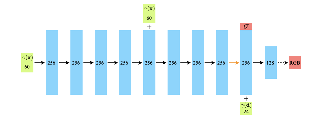
The NeRF architecture is a simple MLP with one residual connection. After the last full-size linear layer, there is a prediction head that predicts the volume density $\sigma$ of the point $\textbf{x}$ in space. At this point, the hidden state is concatenated with the viewing direction $\textbf{d}$; this concatenated output is then used to predict the color $\textbf{c}$ of the point in the space (see the figure below).

Note that, although the NeRF function takes in both position and direction, most of the network only operates on the position. This is to encourage multi-view consistency: regardless of what direction a point is seen from, it should contain the same amount of “stuff.” That is why the predicted volume density does not take viewing direction into account.

The other detail to note, seen in the figure, is that the NeRF uses a positional encoding function $\gamma$. This is similar to the positional encoding used in the original transformer, but in this case the purpose is to map the input position and direction to higher dimensions. In general, doing this makes it easier for multi-layer perceptrons to learn more complex functions.

When training a NeRF, we require camera poses that contain the position and viewing direction information for corresponding input images. Sometimes these are known in advance, but often we need to use some sort of structure-from-motion pipeline to acquire them. COLMAP is one such pipeline that is commonly used—we can give it our images and it will return their poses (unless it fails, which happens sometimes).

We can now generate rays from these camera poses. The idea here is that for input image, we can use its corresponding camera pose to shoot rays into the scene through every pixel we wish to reconstruct. We can then sample points along these rays, pass them into our network (remember that the network takes a point and a direction), and then render a color for each pixel using the network’s output along each ray. We can compare our predicted pixel values against the ground truth pixel values taken from our images to calculate a loss and optimize the network. If some of this is confusing now, it will become intuitive when we cover the volume rendering equation and model optimization in further detail.

Volume Rendering

This is the volume rendering equation that calculates the color for a given ray:

The equation may look complicated if you have never seen it before but it’s actually very interpretable—let’s break it down.

A ray is defined by $\textbf{r}(t) = \textbf{o} + t\textbf{d}$ where $\textbf{o}$ is the origin of the ray, $\textbf{d}$ is the direction of the ray, and $t$ is a scalar. So for any value of $t$, $\textbf{r}(t)$ is a 3D vector representing a position in space.

We can immediately recognize $\sigma(\textbf{r}(t))$ and $\textbf{c}(\textbf{r}(t), \textbf{d})$ in the equation—these are the volume density and color that are predicted by our NeRF in a given forward pass for position $\textbf{r}(t)$ and viewing direction $\textbf{d}$. Intuitively, when the volume density is higher (i.e. there is some object at this point in space), the color of that point will contribute more to the final calculated color of the ray, since those two quantities are multiplied. And similarly, when the volume density is close to zero (i.e. there is nothing at that point in space), that point’s contribution to the final color will be negligible.

The function $T(t)$ is the accumulated transmittance along the ray, which is basically a measure of how much “stuff” has been hit while tracing the ray from $t_n$ to $t$. To visualize its contribution to the final rendered color of the ray, let’s set $u = \int_{t_n}^{t}\sigma(\mathbf{r}(s))ds$. This allows us to write the accumulated transmittance as $T(u) = e^{-u}$, which is just the inverse exponential function.

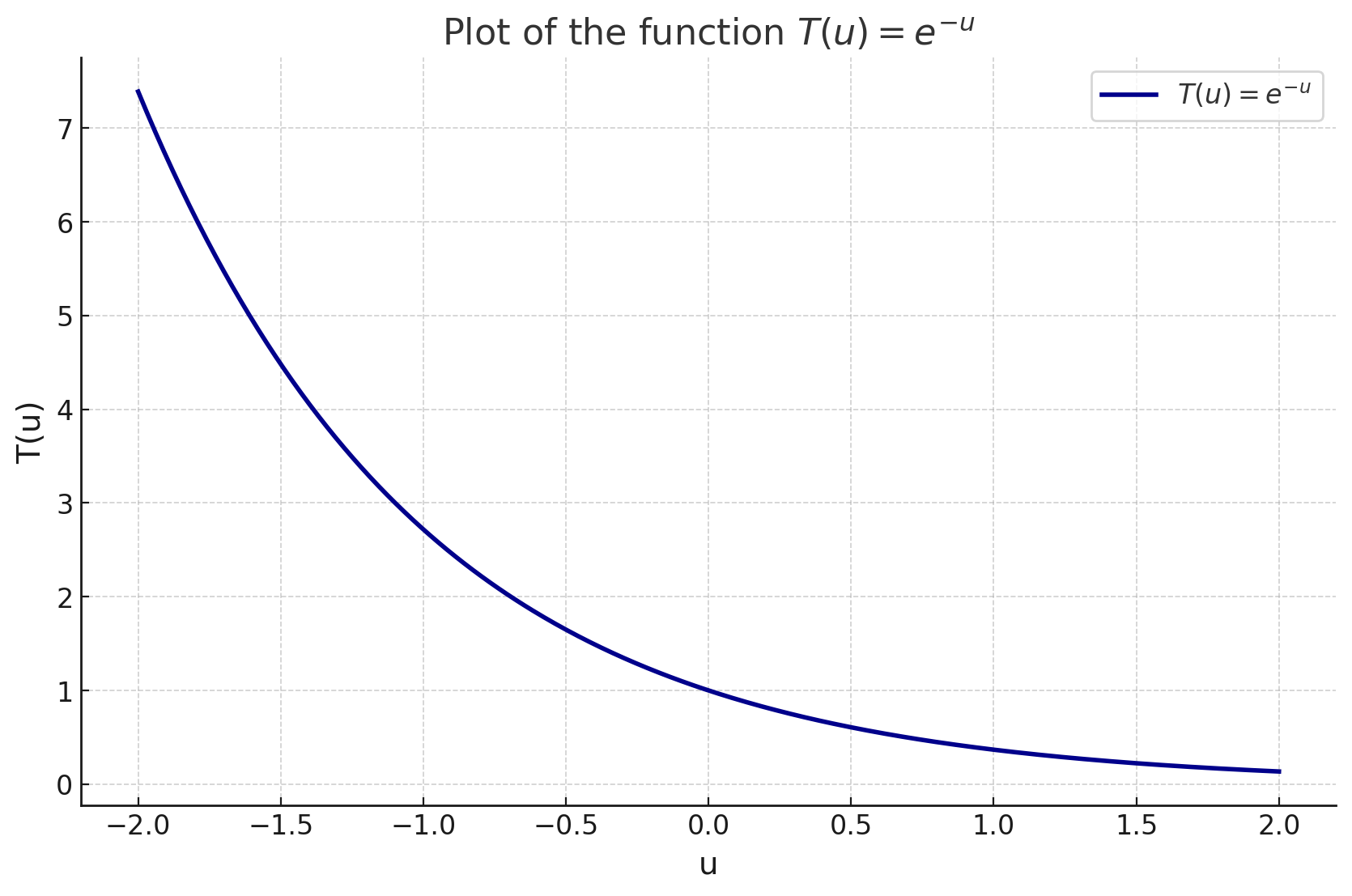
We can see that $u$ is the sum of the volume density of each infinitesimal particle ($ds$) along the ray. Since volume density cannot be negative (physically and in implementation since $\sigma$ is predicted using ReLU), $u$ will always be nonnegative. So the accumulated transmittance value will decrease from 1 as volume density accumulates along the ray. In the context of the volume rendering equation, this makes a lot of sense: once the ray has hit objects, the color contribution of points further along the ray should given less weight, since it is usually hard to see through objects.

We now have mathematical intuition for every part of the volume rendering equation, except for the bounds of the integral. The bounds are straightforward, but I’ll still cover them to illustrate some computational points.

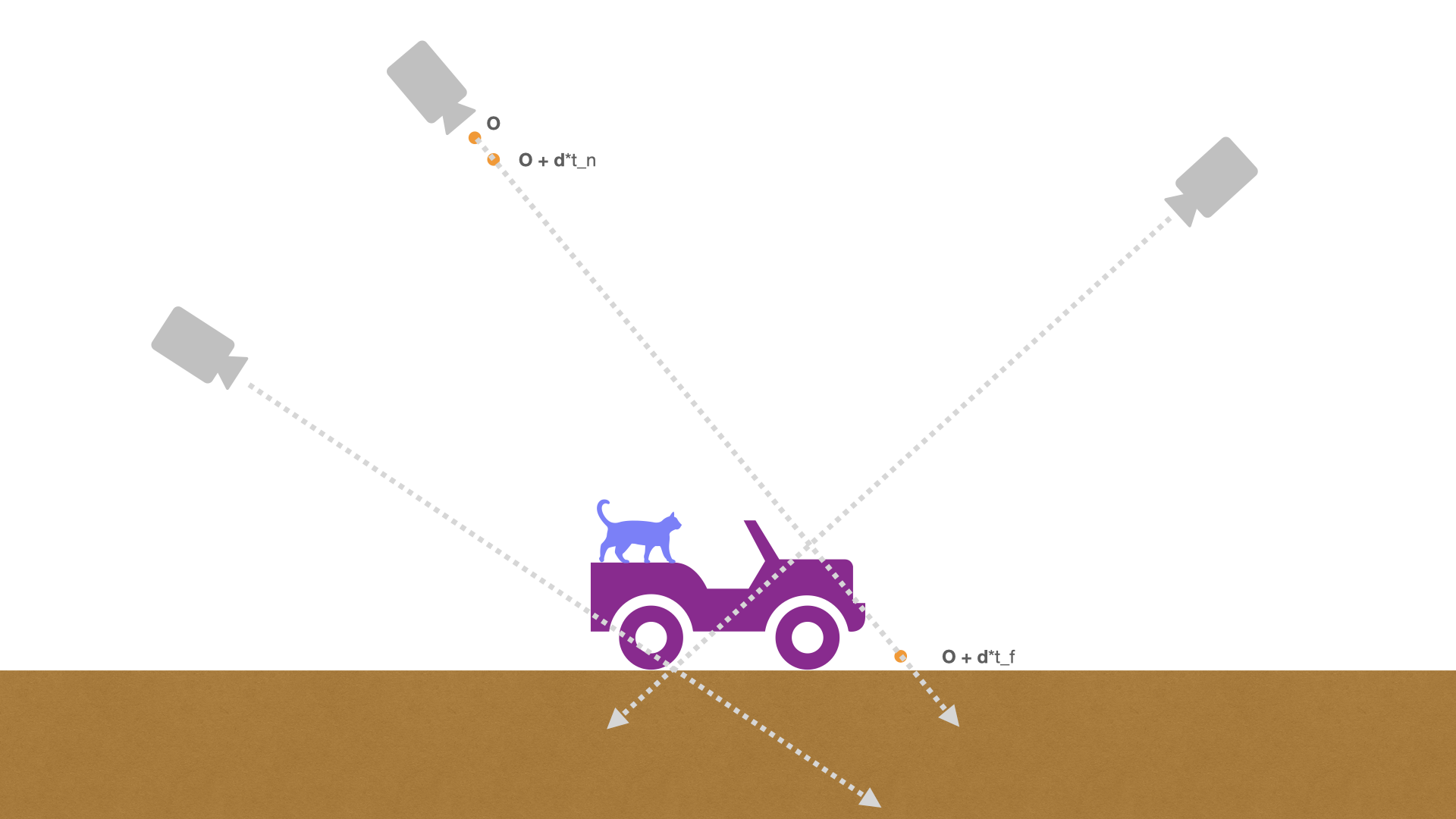
We calculate the integral from a near bound $t_n$ to a far bound $t_f$. To illustrate the importance of the bounds, imagine that we are training a NeRF on scene images taken from a drone high above an object of interest, as in the picture above. If $t_n$ is too small, then we will be running forward passes on points that are pretty much just air, which has near-zero volume density—since volume density is multiplied by color to calculate each point’s color contribution to the final rendered color, these points will effectively have no contribution; this will result in a bunch of wasted computation. Similarly, if $t_f$ is too large, we could be running forward passes on points for which $T(t)$ is very small—more wasted computation.

In implementation, the volume rendering integral is approximated numerically. We split $[t_n, t_f]$ into evenly spaced bins and sample a point uniformly from each bin. The discrete formula is:

where $\delta$ represents the distance between adjacent samples. This is just an implementation detail—the intuition here is the same as before: points with higher volume density contribute more to the rendered color, and contributions decrease as density accumulates along the ray. The difference is just that the integrals are replaced with sums and $\sigma(\mathbf{r}(t))$ has been replaced with $1 - \exp \left(-\sigma_i \delta_i)\right)$.

Hierarchical Sampling

In practice, the authors of the original paper jointly optimize two NeRFs: one “coarse” model and one “fine” model. The reason is that, even if we can pick reasonable $t_n$ and $t_f$ bounds for the scene, we will still be running forward passes on points that have near-zero volume density and points that are occluded; this can be mitigated by training a coarse model whose predictions can inform the fine model how to sample points more effectively.

This joint optimization is accomplished by first taking $N_c$ samples along the ray, running them through the coarse network, and then writing the output as a weighted sum:

Higher $w$ values correspond to a greater contribution to the rendered color. We can normalize these values as $w_i = \frac{w_i}{\sum_{j}^{N_c}w_j}$ to generate a probability distribution where relevant points are weighted higher. Then we can sample $N_f$ points from this distribution. The fine model then runs on these $N_f$ points in addition to the original $N_c$ points.

Optimization

The loss score used for NeRFs is the mean squared error between predicted RGB pixel values and ground truth pixel values. Note that we don’t optimize directly over the output of a single forward pass: for example, in an image classification task, a network predicts a probability distribution of classes for a single image and that predicted distribution is used to directly compute a loss; in the case of NeRFs, we make many predictions, perform volume rendering over them, and then compute the loss based on the output of the volume rendering step.

Subsequent Work

While the vanilla NeRF described in this post was revolutionary, it has its limitations. It tends to do worse when trained on images of varying scales; it suffers from aliasing effects; it has trouble with images taken in different lighting conditions, etc. Improved NeRF models have been created to tackle these issues. In general, there have been many new developments along this line of work. To keep exploring, I suggest the awesome-NeRF repo and Jon Barron’s research website.

References

[1] Mildenhall et al. ”NeRF: Representing Scenes as Neural Radiance Fields for View Synthesis”

[2] Gao et al. ”NeRF: Neural Radiance Field in 3D Vision, A Comprehensive Review”

[3] yenchenlin, nerf-pytorch